Minimal Simulations
As a guideline, we recommend to simulate membranes composed of at least 128 lipids per monolayer, and the analysis to be performed for at least 300 ns (after proper equilibration of a few tens to 100 ns). We also recommend a temporal resolution of one PDB saved every 100 ps (Tutorial) in order to ensure the absence of correlation between the defects from different frames since the lifetime of lipid-packing defects is typically < 20 ps. Using these settings, the user can obtain robust statistics on fluid bilayers using all-atom force fields. For example, a palmitoyl-oleoyl-phosphatidylcholine (POPC) bilayer simulated for 300 ns (after 100 ns of equilibration) displayed 174 599 deep defects. What matter in the end is the total number of defects, if you have more than 150 000 you should be safe. See the section How to interpret barplots? below.
Statistical Analysis
To obtain robust statistics for a given lipid composition and set of conditions, one needs to collect the packing defects from a few thousands of snapshots. After a given equilibration time (typically a few tens to 100 ns), all packing defects from frames separated by 100 ps of a trajectory are determined and their area accumulated in a single vector (for both upper and lower leaflets). From this vector, a histogram of packing defect areas is then computed. The histogram bin width has to be carefully chosen to insure fair comparison between different simulations. Since the grid resolution is 1 Å2, we generally recommend the use of 1 Å2 for the bin width. The lipid-packing defect area follows an exponential distribution and can be conveniently fitted to a mono-exponential decay:
p(A) = b.e-d.A = b.e -A/π
where p(A) is the probability of finding a lipid-packing defect of area A, b is a constant, d is the exponential decay in units of Å-2, and π is the packing defect constant in units of Å2. We generally recommend to use the packing defect constant (instead of the decay) because it is more intuitive: the higher the π constant, the more abundant and the larger the lipid-packing defects. Because very small defects tend to be equally distributed whatever the conditions (e.g. lipid composition, curvature, etc) and defects with low probability converge very slowly, we recommend to perform the fit on defects larger than 15 Å2 and for probabilities ≥10-4.
Error Values
We believe that an error determined by block averaging, as reported here, is reliable and we encourage the users to follow this procedure in the future. The trajectory is divided in 3 equal blocks and the error is the standard deviation over the 3 blocks. Note that each block has to be long enough in order to give robust results.
The statistical significance of the packing defect calculation depends on the size and length of the MD simulations. To obtain reasonable error values by block-averaging (typically below 0.5-0.6 A2 for deep defects), the total number of defects found in the two leaflets has to be at least 105.
Using these rules, for phospholipid bilayers made of a single lipid species:
- πdeep ranges between 6 and 10 Å2,
- πshallow ranges between 7 and 15 Å2,
- πall ranges between 9 and 20 Å2.
How to interpret the barplots?
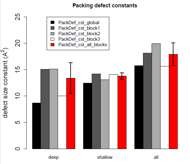
In the tutorial we provide an example that uses a small trajectory of 400 frames. If you could go over the full tutorial, you should have obtained the following barplot:

Example of barplot obtained with the R script on a trajectory of 400 frames.
The first (black) bar correspond to the packing defect constant calculated using all frames of the trajectory. The bars 2, 3 and 4 correspond to the trajectory divided in 3 blocks (dark gray bar: first third, light gray bar: second third, white bar: third third). The last (red) bar correspond to the mean +/- std dev over bars 2, 3 and 4 (thus it provides an error using block averaging with 3 blocks). As can be seen the bars 2, 3 and 4 are not equal and thus lead to a large error. This is clearly indicative of undersampling, the total number of defects is not large enough (in this case, it is between 30000 and 50000, whereas it should be larger than 150000!).
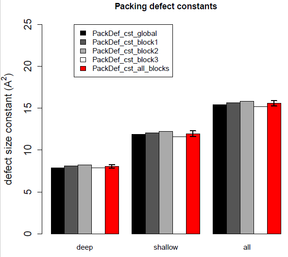
We also provide another example using a trajectory of 3000 frames (300 ns sampled every 100 ps). Note that this comes from the same initial trajectory as the first example, but here we have one frame every 100 ps (instead of one frame every ns). When we run the R script on this example, we obtain the following barplot:

Example of barplot obtained with the R script on a trajectory of 3000 frames.
Here we clearly see that all bars are nearly equal leading to an acceptable error. We thus recommend to carefully assess the total number of defects which should exceed 150000 (typically, a bilayer of 256 lipids and statistics collected on 3000 frames should be OK for a membrane like POPC, see above).
